Interactive model explorer (WIP)
The optional modello.gui module renders nested models in a local browser.
Install its separate extra; the base library still depends only on SymPy:
$ pip install 'modello[gui]'
$ python -m examples.gallery
From a checkout, use uv run --extra gui python -m examples.gallery. Open
http://127.0.0.1:5070. The gallery introduces
scalar models, composition, vectors, and recurrent model states through the
same practical question progression. A separate Extensions page demonstrates
the opt-in stochastic module.
Quickstart: your own explorer
Save this complete example as return_model.py and run
python return_model.py after installing modello[gui]. Open
http://127.0.0.1:5058. From a checkout, the same example runs with
uv run --extra gui python -m examples.gui_quickstart.
from sympy import Rational

from modello import InstanceDummy, Modello
from modello.gui import ModelInfo, Scenario, create_app, gui


@ModelInfo(
    title="Return model",
    description="Explore return and expected gain.",
    initial_field="expected_return",
    highlights=("gain",),
    scenarios=(
        Scenario(
            title="8% return",
            description="Supply a return and calculate expected gain.",
            bindings={"expected_return": Rational(2, 25)},
            select="gain",
        ),
    ),
)
class ReturnModel(Modello):
    expected_return = gui(
        InstanceDummy("return", real=True),
        title="Expected return",
        symbol="μ",
        number_format="percent",
        description="The assumed mean annual arithmetic return.",
    )
    capital = gui(InstanceDummy("capital", positive=True), title="Starting capital", symbol="C", unit="USD")
    gain = gui(capital * expected_return, title="Expected gain", symbol="G", unit="USD")


if __name__ == "__main__":
    app = create_app(ReturnModel, inputs={"capital": 100_000})
    app.run(host="127.0.0.1", port=5058, debug=False)
Capital starts as a supplied input and expected return starts free. Choose 8% return to calculate USD 8,000 expected gain. Change capital to USD 200,000 to see gain update to USD 16,000. Drop the return input to explore the formula again, or supply a gain instead to infer the required return.
Plain model declarations work without presentation metadata. Add gui where
labels, descriptions, symbols, or display formats help. @ModelInfo adds the
model’s text and optional guided questions. Only serving the browser requires
the GUI extra; core annotations and Python snapshots work without Flask.
Choosing what you know
An input is a supplied observation, not a permanent role assigned to a field. You can change an original input, drop it, or supply a normally calculated result as a target. Dropping an observation keeps the defining equations: the quantity may become free, or it may be inferred from other observations. Supplying a target adds an observation; it does not replace its equation or silently discard conflicting inputs.
The Inputs view makes this choice explicit. Checked quantities are supplied; unchecked quantities are left to the model. Edit values, uncheck assumptions, or check a result and enter its target. Apply inputs validates all pending changes together. The results continue to show the last applied case until then. Rejected cases preserve both those results and the pending changes. Discard changes returns the draft to the applied case without solving. The apply controls stay visible while you scroll through pending changes.
The view distinguishes Original, Changed, Added, and Dropped inputs. Each row shows its original supplied value when there was one. Its reset arrow restores that quantity’s original input state in the draft; it does not reset other quantities. Aliases share one observation and one row. Hidden inputs remain active and have no checkbox or editor.
Each guided question restores the initial observations before applying its changes. Subsequent edits remain a custom exploration until you reset inputs.
Vectors and indexed formulas
The explorer recognises declared vectors automatically. Their symbols carry an
arrow, scalar coordinates use subscripts, and values appear as columns. Sums,
products, integrals, derivatives, and limits retain mathematical notation.
An indexed vector definition includes its iteration domain, for example
for i ∈ {0, …, 4}. Sum and product bounds are inclusive, like SymPy limits.
Choose Inspect vector to see its complete values, formula, connected quantities, and individual entry sources. Mixed means its entries have different sources, such as two observations and one inferred result; each entry keeps its own Input, Free, Calculated, or Recorded label.
Supply an entire vector with [1, ?, 3/2]. A ? leaves that entry
unobserved, retaining its equation. Percentages are accepted per entry, such as
[10%, ?, -2%]. Applying a vector checks all entries together. Subsequent
individual edits compose with that proposal. Drop observations releases
the whole vector, and Restore original input restores its original
observation pattern. The Inputs view also supports changing coordinates
together with other model observations.
Whole-vector editing is available when all its coordinates can be edited.
Hidden entries are omitted from summaries and disable whole-vector editing;
Recorded entries retain their snapshot policy. Visible coordinates remain
independently inspectable. Vector metadata supplies default labels, units, and
number formatting to entries; explicit coordinate metadata replaces that
default. Python initial inputs and scenarios accept vectors or sequences at a
vector path, including nested paths such as "window.samples". The browser
uses bracketed coordinate paths such as "window.samples[2]".
An entry’s View in equations action opens the complete indexed vector
definition, including when the entry was reached through an alias.
Understanding the interface
The colour key describes the source of a quantity, independently of whether its current value is numeric or symbolic:
Input is a supplied observation. It can be edited or released.
Free is an open quantity still represented by its own symbol.
Calculated follows from the model’s equations. A numeric result stays calculated and updates when its inputs change. A result can also be observed as a target, making it an input instead.
Recorded is a copied component result retained in a recorded problem. Its editor is disabled because that observation is held in the snapshot.
Hover or focus a colour key to read its explanation. Touch users can tap a key; tap elsewhere or press Escape to dismiss it. The case-status key also explains the distinction between a symbolic preview and a checked numerical case. Colour is accompanied by text labels throughout.
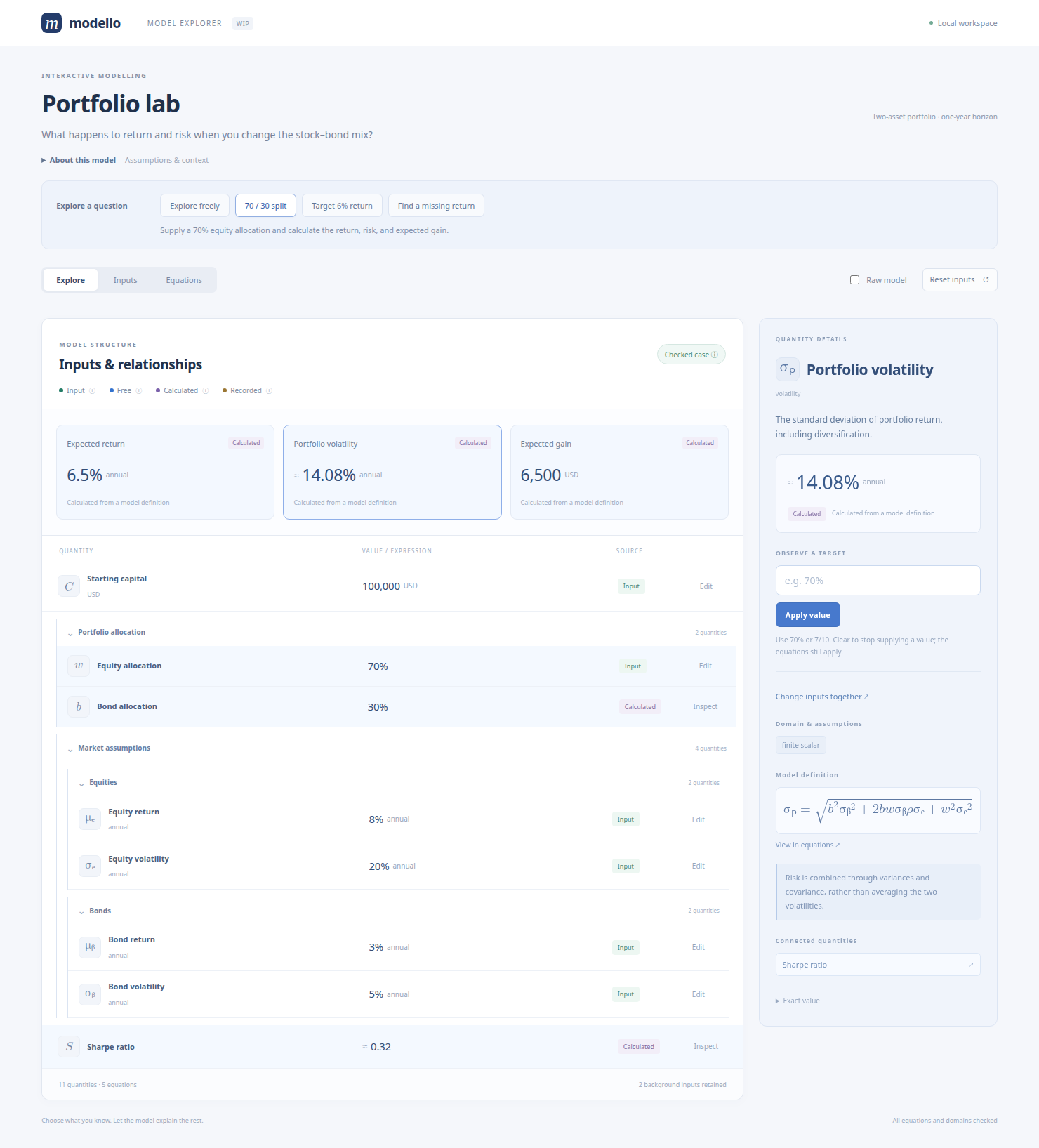
The inspector shows descriptions, units, source, domain chips, mathematical definitions, and links to connected quantities. Expressions use native MathML instead of printed Python or diagnostic constraint lines. Open View in equations for a definition that needs more room. Numeric displays use compact rounded values; an approximation sign marks rounding, and Exact value retains the underlying expression in the displayed units.
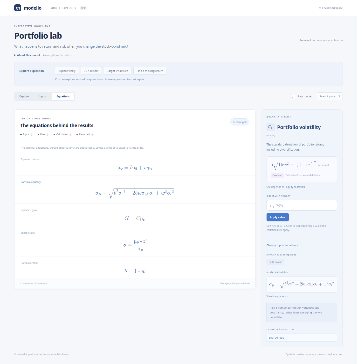
Raw model shows definitions without invoking the solver, retaining recorded inputs in the editor. Equations shows the original defining equations before observations are substituted. Hover, focus, or tap a symbol to inspect its path and description. Tab, Enter, and Space support keyboard exploration.
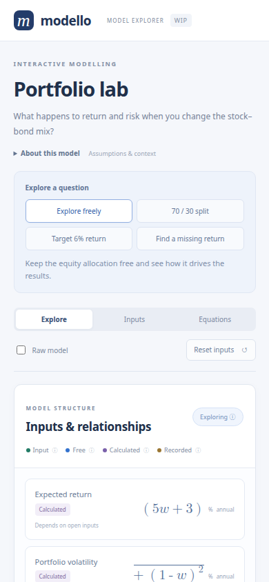
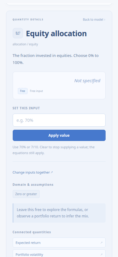
On narrow screens the inspector moves below the model. Selecting a quantity brings its details into view; Back to model returns to the quantities. Tooltip placement is clamped to the viewport.
Starting from your model
create_app accepts a model class, an existing instance, or a recorded
ModelProblem. Initial inputs use full dotted paths:
from modello.gui import create_app
from examples.gui import Portfolio, DEMO_INPUTS

app = create_app(Portfolio, "My portfolio", inputs=DEMO_INPUTS)
app.run(host="127.0.0.1", port=5058, debug=False)
With an instance, original inputs are reopened as observations and solved outputs are recomputed when inputs change. An overwritten instance field becomes an input, as with component copies. The source instance is never mutated. With a recorded problem, all its constraints remain, including inferred component observations. Those are labelled Recorded and held fixed. Reopen the instance when you want its outputs to recompute from original inputs. Each browser holds its own edits and cannot change another browser’s state.
Descriptions, units, and guided questions
Place presentation beside a field with gui(field, *, ...), as in the
quickstart. All metadata arguments are keyword-only, including direct
FieldInfo(...), ModelInfo(...), and Scenario(...) construction.
gui accepts an InstanceDummy, a calculated expression, or
component(Child). Decorate the class with @ModelInfo(...) for model-level
text and guided questions.
Use gui around the entire value assigned inside a Modello class body:
gain = gui(capital * expected_return, title="Expected gain"). The class
namespace unwraps the declaration before later expressions use the field
normally. This declaration helper is not an arithmetic wrapper; putting
gui(capital, ...) inside a larger calculation, or using its return value
outside that class scope, leaves the declaration uncollected.
Field metadata is a FieldInfo annotation. The core collects it through
the general Annotation mechanism; the solver never receives
GUI wrappers or metadata. Registry lookups are independent of Flask:
from modello.gui import FieldInfo

info = ReturnModel.__modello_annotations__[FieldInfo]["expected_return"]
assert info.title == "Expected return"
# A typed helper for extension consumers:
assert FieldInfo.for_model(ReturnModel)["expected_return"].symbol == "μ"
assert ModelInfo.for_model(ReturnModel)[""].title == "Return model"
Nested annotation paths are scoped automatically, such as
"market.equity.expected_return". Components retain their own declarations;
gui(component(Child), ...) labels that component in its parent. Class
docstrings supply default model and component descriptions. Model classes and
component instance types are preserved. See Extension annotations for
writing other extensions using the same registry.
For models declared elsewhere, a ModelInfo(fields=...) mapping can override
presentation by relative dotted path. Application-level metadata= overrides
take priority over that mapping, followed by inline annotations. Each override
replaces the whole FieldInfo for that path. Model presentation uses the
annotation registry; __gui__ blocks are rejected with a migration hint.
Presentation never changes the algebra.
highlights makes selected quantities prominent as result cards.
initial_field chooses the first inspector selection. A Scenario contains
trusted scalar observations and an optional field to select. Paths and edit
permissions are validated; a scenario cannot change hidden or Recorded values.
Its observations still pass through the same validation as manual edits.
Use None in a scenario’s bindings to drop a specific initial observation;
other initial observations remain active.
Presentation paths are checked when constructing Explorer or create_app,
before serving any requests. Errors name the offending option or scenario,
include the full nested path, and suggest similar field names when available.
For example, a misspelt Scenario(title="Target", ...,
select="expected_retrn") reports Scenario 'Target'.select and suggests
'expected_return'. Initial input paths and snapshot bindings use the same
path checks. A scenario targeting hidden or Recorded data explains why the
quantity cannot be edited.
Repeating gui metadata on the same field or
ModelInfo on the same class raises ModelDefinitionError; subclasses
can explicitly refine inherited presentation in their own declaration scope.
symbol is literal text, including Unicode, rather than LaTeX. unit is a
display label without automatic unit conversion or dimensional analysis.
number_format="percent" displays fractional values in percent and seeds
the editor with percentage notation. Numeric summaries do not change exact
values or loosen validation.
A hidden field or component has no row or editor. Its original inputs remain in every solve, and the browser cannot replace or release them, including through aliases. Hidden observation values are omitted from the browser response; their public symbols and descriptions remain inspectable in formulas. This is presentation rather than a secrecy boundary: derived outputs and public model notes can reveal inputs.
Exact edits and validation
Editors accept numbers, +, -, *, /, **, sqrt(...), pi,
E, and I. A trailing % divides the whole expression by 100:
70% and 7/10 are the same exact value. 1.25 is exactly 5/4.
Input length, literal and arithmetic sizes, and powers are bounded. The parser
uses Python’s syntax tree without evaluating Python or SymPy expression strings.
Arbitrary functions, attribute access, and new parameter names are not accepted.
The trusted Python API continues to accept normal symbolic scalar inputs.
Vector and request budgets scale with the declared, trusted model shape; each entry retains the scalar arithmetic limits. Accepted input expressions are kept as editor text, even when their exact values expand to much longer fractions or integers. This lets a later coordinate edit reuse the applied proposal without turning an accepted expression into an oversized literal.
The proposed case is checked against original equations and all declared assumptions, including domains of calculated and hidden quantities. Invalid edits identify both the edited fields and any derived domain failures, while retaining the last successful model. No arbitrary branch or sampled point is chosen when several solutions remain.
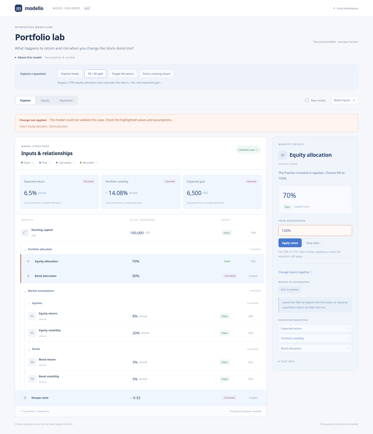
A unique symbolic proposal is labelled Exploring when its audit cannot establish a fully checked numeric case. This includes partially bound models and unresolved external parameters. It is not a claim that every remaining parameter value is admissible. Checked case requires a closed candidate satisfying every audit. Failure to produce a solver candidate is reported as failure to validate a case, not as proof of inconsistency.
Scope of this draft
The interface serves bundled HTML, CSS, JavaScript, MathML, and the STIX Two Math font without a CDN or JavaScript build. The local Flask server is intended for small trusted models on loopback. Symbolic work is synchronous; arithmetic limits are not a solver timeout. There is no deployment, authentication, persistence, multi-branch selection, or model-instance export flow.
Construction and the preview share directed-definition expansion and candidate
generation. The preview uses the diagnostic audit while construction retains
its original filtering. Python users can call Explorer(...).snapshot(raw=True)
for a solver-free, JSON-ready view without installing Flask. Snapshot kind
uses derived for both numeric and symbolic calculations and fixed only
for recorded component observations; value_state describes the display form.
Each visible field also reports initial_input and an input_state of
initial, overridden, added, dropped, or unspecified. This input
history is independent of whether the current value is free or calculated.
Hidden fields omit original values and report input_state="hidden".
Python snapshots are stateless proposals against the initial observations:
snapshot({"height": 6}) overrides height, and snapshot({"height": None})
drops it. Omitting height from the next proposal restores its original state.
Pass all desired overrides and drops together in one mapping. The browser
retains this mapping between edits and removes a field’s override when you
restore it individually.
Typed model vectors
The account gallery model nests typed executions and
account states under their vectors. Add or remove executions, inspect a member,
and edit its quantities. The source recurrence appears once; calculated fields
link back to it. Patterns such as fills[] and fills[].price provide
member labels and indexed symbols.
ExplorerValue covers scalar, vector, and model-vector observations. For the
Python API, ModelVectorInput supplies ordered records such as
{"fills": [{"quantity": 2, "price": 100, "fee": 1}]} alongside scalar
paths such as "states[0].cash". Record length determines the window.
Mathematical rendering
Native MathML renders vector arrows, subscripts, Σ/Π/∫, and stretchy brackets
using the locally bundled STIX Two Math font. Expectation, variance, and the
process generator use 𝔼, 𝕍, and ℒ. LaTeX export uses the corresponding
mathematical alphabets. Font attribution and its SIL Open Font License are
bundled under modello/_gui/static/fonts/.
API
Optional local exploration of nested models (install modello[gui]).
Presentation metadata never changes the algebra. Raw snapshots do not solve; browser edits are exact scalars parsed without evaluating expression strings.
- exception modello.gui.BindingError(message: str, paths: tuple[str, ...] = ())
A rejected edit, with field paths that the interface can highlight.
- class modello.gui.Explorer(model: type[Modello] | Modello | ModelProblem, name: str = 'exploration', *, inputs: Mapping[str, SymbolicScalar | int | float | complex | str | Decimal | Fraction | Vector | Sequence[SymbolicScalar | int | float | complex | str | Decimal | Fraction | None] | SymbolicVector | Sequence[Mapping[str, SymbolicScalar | int | float | complex | str | Decimal | Fraction | None] | None]] | None = None, metadata: Mapping[str, FieldInfo] | None = None)
Prepare raw or bound views of a class, instance, or recorded problem.
Declare model text with
@ModelInfo(...)and field labels withgui. Component declarations are inherited by the layout;metadataoverrides field or component labels by full dotted path.inputssupplies initial bindings by dotted path. The original model instance is never mutated.- snapshot(bindings: Mapping[str, SymbolicScalar | int | float | complex | str | Decimal | Fraction | Vector | Sequence[SymbolicScalar | int | float | complex | str | Decimal | Fraction | None] | SymbolicVector | Sequence[Mapping[str, SymbolicScalar | int | float | complex | str | Decimal | Fraction | None] | None] | None] | None = None, *, raw: bool = False) dict[str, Any]
Return a JSON-ready view; invalid edits raise without changing state.
Bindings replace initial inputs, and
Nonedrops an observation without removing definitions. Omit a path to restore its initial input state. Several bindings are checked together as one proposed case. Raw views show definitions without solving. Bound views label an undecided audit as a conditional preview.
- class modello.gui.FieldInfo(*, title: str = '', description: str = '', info: str = '', symbol: str = '', hidden: bool = False, unit: str = '', number_format: Literal['number', 'percent'] = 'number')
Display metadata for a scalar or component, without changing its algebra.
All metadata arguments are keyword-only.
symbolis literal MathML text, not LaTeX.hiddenremoves the editor and observation value while retaining its inputs. Calculated outputs can still reveal input values; hiding is a presentation choice.unitis a display label;number_format='percent'renders fractions as percentages.
- class modello.gui.ModelInfo(*, title: str = '', description: str = '', info: str = '', fields: Mapping[str, ~modello.gui.FieldInfo]=<factory>, highlights: tuple[str, ...]=(), initial_field: str = '', scenarios: tuple[~modello.gui.Scenario, ...]=())
Decorate a model with its text and exploration hints.
Use
@ModelInfo(title=..., ...)above the class. Declare field metadata inline withgui. Optionalfieldskeys are relative dotted paths for presentation overrides, including labels on components from other models.highlightsselects result cards,initial_fieldopens an inspector, andscenariossupplies named explorations from the initial inputs. All metadata arguments are keyword-only.
- class modello.gui.Scenario(*, title: str, description: str, bindings: Mapping[str, ~modello._values.SymbolicScalar | int | float | complex | str | ~decimal.Decimal | ~fractions.Fraction | ~modello.vectors.Vector | ~collections.abc.Sequence[~modello._values.SymbolicScalar | int | float | complex | str | ~decimal.Decimal | ~fractions.Fraction | None] | ~modello._values.SymbolicVector | ~collections.abc.Sequence[~collections.abc.Mapping[str, ~modello._values.SymbolicScalar | int | float | complex | str | ~decimal.Decimal | ~fractions.Fraction | None] | None] | None]=<factory>, select: str = '')
A named exploration that restores initial inputs, then applies bindings.
All arguments are named. Only visible, editable quantities may be bound.
selectopens a field in the inspector; it need not be the quantity being observed.
- modello.gui.create_app(model: type[Modello] | Modello | ModelProblem, name: str = 'exploration', *, inputs: Mapping[str, ExplorerValue] | None = None, metadata: Mapping[str, FieldInfo] | None = None) Flask
Create a local Flask app; each browser holds its own trial bindings.
Serve with
app.run(host='127.0.0.1', debug=False). The bundled frontend needs no CDN, JavaScript build, or external math renderer. The prototype runs symbolic work synchronously and is intended for small local models.
- modello.gui.gui(field: _ValueT, *, title: str = '', description: str = '', info: str = '', symbol: str = '', hidden: bool = False, unit: str = '', number_format: Literal['number', 'percent'] = 'number') _ValueT
Annotate a scalar or component declaration without changing its type.
Wrap the entire assigned value:
field = gui(expression, title=...)inside a Modello class body. The class namespace unwraps the declaration before later expressions use it; this helper is not an arithmetic wrapper outside that scope. Metadata is stored underModel.__modello_annotations__[FieldInfo].