How much time should we spend checking a record?
An archive is digitising paper records. Typing faster increases its daily output, but mistakes create work later. A colleague can spend time checking each entry before it leaves the team. How much checking is worthwhile?
Start by following a record through the process:
        flowchart TD
    accTitle: A record's path through checking
    accDescr: Every record is reviewed. Initially correct records stay correct. Errors are either corrected during checking or left for later repair.
    record["Enter a record"] -->|Correct| correct_review
    record -->|Incorrect| error_review
    subgraph review["Review every record"]
        correct_review["Check a correct record"]
        error_review["Check an incorrect record"]
    end
    correct_review --> correct_to_correct["Correct before and after"]
    error_review -->|Caught| corrected["Corrected"]
    error_review -->|Missed| remaining["Still incorrect"]
    remaining --> repair["Later repair"]
Three groups leave checking: correct before and after, corrected, and still incorrect.
This first model assumes that checking introduces no errors. Correcting an error during checking takes no staff minutes beyond the checking minutes already counted. Only records still incorrect after checking need the later repair. The three groups keep track of each record’s path through the process.
One model will answer several questions:
What fraction of records leave checking correct or still incorrect?
What happens as checking minutes grow, or the same short check is repeated?
Which checking minutes minimise total staff minutes per record?
How many records fit within a staff-minutes budget?
We will build a workload model, use calculus to propose a checking time, and check the properties that justify that decision. Then we will change the checking response and revisit the result. You need Python and undergraduate calculus; we explain the concavity argument as we use it. Start modelling introduces Modello’s declarations and observations.
The executable example is examples.record_review. Its symbolic calculations
need only the ordinary modello installation. Every input below is
illustrative: verifying the mathematics does not establish that the chosen
response curve describes a real team.
Start with the workload budget
Start with a familiar identity: staff minutes equal records multiplied by minutes per record. Declare that relationship as an ordinary Modello model:
from modello import InstanceDummy, Modello
class EntryBudget(Modello):
    """Staff minutes = records * minutes per record; supply any two quantities."""

    records = InstanceDummy("n", positive=True)
    minutes_per_record = InstanceDummy("m", positive=True)
    staff_minutes = records * minutes_per_record
Each InstanceDummy names a quantity whose value can be supplied or inferred.
records is the field name used for inputs; "n" is its symbolic label.
These two quantities are positive. We can supply values on either side of the
equation. The examples below import this declaration; the first argument to
EntryBudget names the instance.
>>> from examples.record_review import EntryBudget
>>> day = EntryBudget("day", staff_minutes=480, minutes_per_record=4)
>>> day.records
120
>>> target = EntryBudget("target", records=150, minutes_per_record=4)
>>> target.staff_minutes
600
Staff time adds across the team: two people working for 240 minutes each provide 480 staff minutes. We use a continuous record count as a planning estimate. So far we have counted only typing; checking and later repairs must come from the same pool of staff time.
Model a short check
Suppose typing takes four minutes per record. One in ten records has an error that takes sixty staff minutes to repair. We count at most one error per record. Without checking, repairs therefore add \((1/10)\times60=6\) minutes per record in expectation. Total expected work is ten minutes per record, giving capacity of 48 records per 480 staff minutes under this workload approximation.
Keep these estimates and their repair-work relationship in a model that we can reuse for both a short check and the final plan:
class RecordWork(Modello):
    """Entry and expected repair minutes per record before checking."""

    entry_minutes_per_record = InstanceDummy("b", positive=True)
    error_fraction = InstanceDummy("p", nonnegative=True)
    repair_minutes_per_error = InstanceDummy("L", positive=True)
    repair_minutes_per_record = error_fraction * repair_minutes_per_error
    minutes_per_record = entry_minutes_per_record + repair_minutes_per_record
>>> from sympy import Rational
>>> from examples.record_review import RecordWork
>>> record = RecordWork("record", entry_minutes_per_record=4,
...                     error_fraction=Rational(1, 10), repair_minutes_per_error=60)
>>> record.repair_minutes_per_record, record.minutes_per_record
(6, 10)
The names state the units: repair_minutes_per_error is the duration of one
repair. Multiplying by error_fraction gives the expected
repair_minutes_per_record. Adding entry_minutes_per_record gives the
total minutes_per_record before checking.
How might checking reduce that repair work? Start with a short check and assume a constant detection rate. A short check catches a proportion of the errors still left, approximately the detection rate multiplied by the checking minutes. For example, a detection rate of one half per minute means a six-second check catches about five percent of the errors present at the start of that check.
The same short check then catches fewer errors on a second pass, because fewer remain. This is our modelling assumption about diminishing returns. It describes how checking might work; we would need measurements to assess it.
Reuse these estimates as a record component in the short-check model.
component(RecordWork) gives it the record’s quantities, such as
record.error_fraction. The other inputs are checking minutes per record and
the detection rate:
from modello import component
class CheckingStep(Modello):
    """Approximate a short check that catches a share of the errors still left.

    Physical inputs need record.error_fraction <= 1 and 0 <= detection_rate * minutes_per_record <= 1.
    These are modelling assumptions here, not automatically checked bounds.
    """

    record = component(RecordWork)
    minutes_per_record = InstanceDummy("h", nonnegative=True)
    detection_rate = InstanceDummy("k", real=True)
    caught_share = detection_rate * minutes_per_record
    remaining_share = 1 - caught_share
    remaining_error_fraction = record.error_fraction * remaining_share
    repair_minutes_per_record = remaining_error_fraction * record.repair_minutes_per_error
caught_share is a fraction of the errors present at the start of the step.
remaining_error_fraction is a fraction of all records. With our inputs:
>>> from examples.record_review import CheckingStep
>>> short = CheckingStep("short", record=record, minutes_per_record=Rational(1, 10),
...                      detection_rate=Rational(1, 2))
>>> short.caught_share
1/20
>>> 1000 * short.remaining_error_fraction
95
>>> short.record.repair_minutes_per_record
6
Out of an illustrative 1,000 records, 100 initially need repair; the short check is expected to catch five and leave 95. The last output recovers our six expected repair minutes per record before checking. The error fraction must lie between zero and one, and a step must be short enough that its caught share also lies between zero and one. This ordinary model records the relationships; it does not enforce those bounds.
Build up a longer check
To describe a longer check, divide its total time \(t\geq0\) into \(N\) equal steps. Write \(k\) for the constant detection rate, measured per minute. Each step lasts \(t/N\) minutes and leaves the fraction \(1-kt/N\) of the errors it started with. After two steps we multiply that fraction by itself; after \(N\) steps the fraction still missed is \((1-kt/N)^N\).
Use the same Modello declaration with symbolic inputs, then let SymPy take the limit as the steps become shorter and more numerous:
>>> from sympy import S, Symbol, limit
>>> t = Symbol("t", nonnegative=True)
>>> k = Symbol("k", positive=True)
>>> N = Symbol("N", integer=True, positive=True)
>>> part = CheckingStep("part", minutes_per_record=t/N, detection_rate=k)
>>> part.remaining_share
1 - k*t/N
>>> remaining = limit(part.remaining_share**N, N, S.Infinity)
>>> remaining
exp(-k*t)
>>> 1 - remaining
1 - exp(-k*t)
We have derived a continuous response from our short-step assumption. Write \(u(t)\) for the fraction of the original errors caught after checking for \(t\) minutes:
With no checking, no errors are caught. More checking catches more, but the gain shrinks as fewer errors remain. For a positive detection rate the caught fraction approaches one. SymPy has derived a consequence of our assumption; it has not validated the assumption.
Note
Expressing the repeated checks as a recursive sequence
If your model is naturally recursive, you can declare the update instead
of writing the power explicitly. Start with a remaining share of one: all
original errors are still present. Each check multiplies the previous
share by part.remaining_share.
Modello’s Series and Recurrence express that process:
>>> from modello import Index, Recurrence, Series
>>> j = Index("j", nonnegative=True)
>>> R = Series("R", j)
>>> law = Recurrence(R[j], part.remaining_share * R[j - 1], initial={0: 1})
>>> law.at(0).doit()
1
>>> 1 - limit(law.at(N).doit(), N, S.Infinity)
1 - exp(-k*t)
Here j counts completed checks within one sequence; N is its fixed
total number of checks. law.at(N).doit() derives the expression after
those updates, which we then pass to limit. The geometric power is a
result of the recurrence, giving another way to derive the same response.
You can also use SymPy’s RecursiveSeq directly with the same short-step expression:
>>> from sympy import Function, rsolve
>>> from sympy.series.sequences import RecursiveSeq
>>> i = Symbol("i", integer=True, nonnegative=True)
>>> r = Function("r")
>>> sequence = RecursiveSeq(part.remaining_share * r(i - 1), r(i), i, [1])
>>> sequence[:3]
[1, 1 - k*t/N, (1 - k*t/N)**2]
>>> formula = rsolve(sequence.recurrence, sequence.yn, {r(0): 1})
>>> 1 - limit(formula.subs(i, N), N, S.Infinity)
1 - exp(-k*t)
RecursiveSeq computes individual terms; rsolve
finds a closed form for this linear recurrence. Both routes use the same
initial value and transition, and give the same continuous response.
Reuse the derivation
We will need this response when we build the workload model. Put the calculation
into an ordinary Python function,
derive_checking_response(minutes_per_record, detection_rate). Its arguments
use the same names as the short-check model: minutes_per_record is the
checking duration \(t\), and detection_rate is \(k\), measured per
minute. It returns a SymPy expression for the share of the original errors caught.
The initial error fraction and repair cost enter later, when we convert that
caught share into saved minutes.
The function follows the steps above: divide the checking minutes among short
checks, take the limit of the share still missed, then subtract that share from one.
Its temporary count steps plays the role of \(N\). SymPy’s Dummy
gives that count a fresh symbol so it cannot clash with the input symbols;
Expr is the SymPy expression type used in the type annotations.
from sympy import Dummy, Expr, S, limit
def derive_checking_response(minutes_per_record: Expr, detection_rate: Expr) -> Expr:
    """Derive the caught share from the checking minutes per record and detection rate."""
    steps = Dummy("N", integer=True, positive=True)
    step = CheckingStep("part", minutes_per_record=minutes_per_record / steps, detection_rate=detection_rate)
    remaining_share = limit(step.remaining_share**steps, steps, S.Infinity)
    return 1 - remaining_share
The example module contains this definition. Import it and check that it returns the response we derived above:
>>> from examples.record_review import derive_checking_response
>>> response = derive_checking_response(t, k)
>>> response
1 - exp(-k*t)
>>> response == 1 - remaining
True
Both inputs can remain symbolic. The result is an expression in those symbols, ready to use as a field in another model.
Count the benefit and cost in minutes
We assume that a caught error needs no further repair time beyond the checking
time already counted. If the initial error fraction is \(p\) and a repair
takes \(L\) minutes, checking leaves expected repair work
\(pL(1-u(t))\) per record. The product \(pL\) is exactly the
record.repair_minutes_per_record field we calculated above.
Let \(b\) be entry time and \(a\) be the expected repair work that perfect checking could avoid. Our illustrative inputs are:
Quantity |
Field |
Meaning |
Value |
|---|---|---|---|
\(b\) |
|
Entry minutes per record |
4 minutes per record |
\(a\) |
|
Expected repair minutes per record before checking |
6 minutes per record |
\(k\) |
|
Detection rate |
\(1/2\) per minute |
Now use minutes as the common unit for benefit and cost:
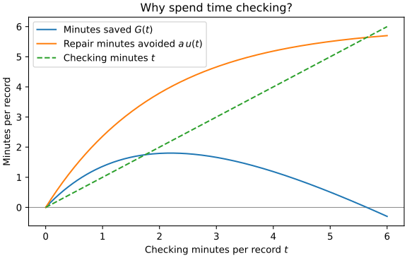
Here \(G(t)\) is minutes saved, the staff time saved compared with no checking. \(M(t)\) is total expected staff time per record. Maximising \(G\) minimises \(M\). Avoided repair minutes give us a concrete measure of utility, in the same units as the checking cost.
The plot labels pair these names with their expressions: repair minutes avoided is \(a\,u(t)\), checking minutes is \(t\), and minutes saved is \(G(t)=a\,u(t)-t\).
State what the calculation needs
Three distinct properties matter:
Strict increase: more checking should catch a larger fraction of errors.
Concavity: the marginal benefit should not increase. When the function for minutes saved is concave, a point with zero derivative is a global maximum.
C² regularity: the first two derivatives should be continuous. We will use a second-order approximation to describe workload near the chosen time.
For the exponential curve, ordinary calculus gives \(u'(t)=ke^{-kt}\) and \(u''(t)=-k^2e^{-kt}\). Its increase needs \(k>0\); concavity and C² regularity hold for every real \(k\). These are separate mathematical facts. A smooth curve can still be a poor description of checking.
A property we ask the checker to establish is a proof obligation.
specifies attaches obligations to a field. VerificationModel attempts
them when the class is defined, retaining each result for inspection.
In the declaration below, minutes_per_record and detection_rate are
InstanceDummy inputs for checking minutes \(t\) and detection rate
\(k\). We can supply checking minutes or keep them symbolic to study the
whole response curve. Although our story expects a positive detection rate,
we leave it unrestricted so the checker can tell us which values establish
the requested properties.
The caught_share field calls
derive_checking_response(minutes_per_record, detection_rate). This is
the function we built from the short-step model, now using the model’s symbols for \(t\)
and \(k\). specifies pairs its returned expression with the three
requested properties.
introduced_error_share uses the same derivation with an
error_creation_rate. We will initially observe that rate as zero to model
checking that creates no errors, then revisit that observation later.
Field paths use the Python attribute names: wrt="minutes_per_record" selects
\(t\). CHECKING_MINUTES_DOMAIN is
the interval of nonnegative checking minutes, so the claims concern every
\(t\geq0\). With the function above already defined, add these imports and
the domain for the verification declaration:
from sympy import Interval, S
from modello import InstanceDummy
from modello.contrib.verification import (
    VerificationModel, concave, continuously_differentiable,
    specifies, strictly_increasing,
)

CHECKING_MINUTES_DOMAIN = Interval(0, S.Infinity)
class ExponentialReview(VerificationModel):
    """Constant-rate correction and error-introduction responses.

    ``minutes_per_record`` measures checking; ``detection_rate`` is per minute.
    The detection rate is deliberately real: increasing response needs it > 0.
    The nonnegative error-creation rate is zero in the baseline scenario.
    The curve follows from a constant detection rate for errors still left;
    that assumption has not been fitted or validated against a real team.
    """

    minutes_per_record = InstanceDummy("t", nonnegative=True)
    detection_rate = InstanceDummy("k", real=True)
    error_creation_rate = InstanceDummy("r", nonnegative=True)
    introduced_error_share = derive_checking_response(minutes_per_record, error_creation_rate)
    caught_share = specifies(
        derive_checking_response(minutes_per_record, detection_rate),
        strictly_increasing(
            "caught_share",
            wrt="minutes_per_record",
            domain=CHECKING_MINUTES_DOMAIN,
            reason="Extra checking must catch a larger fraction of the missed errors.",
        ),
        concave(
            "caught_share",
            wrt="minutes_per_record",
            domain=CHECKING_MINUTES_DOMAIN,
            reason="The marginal benefit must not increase.",
        ),
        continuously_differentiable(
            "caught_share",
            wrt="minutes_per_record",
            domain=CHECKING_MINUTES_DOMAIN,
            order=2,
            reason="The plan approximates total minutes per record near the chosen checking minutes to second order.",
        ),
    )
definition_report() contains the results of those checks. explain(id)
selects one result: caught_share/strictly_increasing combines the field path
caught_share with the obligation’s name. The commands below import the class
whose declaration we have just read.
>>> from examples.record_review import ExponentialReview
>>> definition = ExponentialReview.definition_report()
>>> definition.explain("caught_share/strictly_increasing").verdict
'conditionally true'
>>> definition.explain("caught_share/concave").verdict
'strictly true'
>>> definition.explain("caught_share/continuously_differentiable").verdict
'strictly true'
A verdict concerns the stated domain and the available definitions, data,
and assumptions. strictly true means established. conditionally true
retains a sufficient parameter condition; we will inspect it next.
strictly false means the checker established a failure. unresolved
means the attempt established neither the claim nor its failure.
Find the parameter condition
A VerificationContext holds the definitions, observations, and assumptions
for one branch of the investigation. Its methods return new contexts, leaving
earlier branches available for comparison. Inspect the parameter condition
using the symbols that belong to this context, then add it as an assumption:
>>> from modello.contrib.verification import VerificationContext
>>> curve = VerificationContext.for_model(ExponentialReview)
>>> increase = curve.explain("caught_share/strictly_increasing")
>>> increase.condition == (curve.symbols.detection_rate > 0)
True
>>> positive_detection_rate = curve.assume(curve.symbols.detection_rate > 0)
>>> positive_detection_rate.explain("caught_share/strictly_increasing").verdict
'strictly true'
An assumption restricts allowed parameter values; an observation fixes a value
for a particular branch. SymPy’s Rational(1, 2) keeps the observed detection rate as
an exact fraction:
>>> from sympy import Rational
>>> curve.observe(detection_rate=Rational(1, 2)).explain("caught_share/strictly_increasing").verdict
'strictly true'
With zero detection rate, the curve is constant and the strict increase claim fails:
>>> curve.observe(detection_rate=0).explain("caught_share/strictly_increasing").verdict
'strictly false'
>>> curve.explain("caught_share/strictly_increasing").verdict
'conditionally true'
The earlier context is unchanged. Observations accumulate; to compare different values, branch from the common context before either value was supplied. The reference covers removing assumptions when you need to reopen an earlier choice.
Compose the decision model
Keep the record outcomes in a reusable ReviewModel.
Its record component supplies entry time, avoidable repair work, and baseline
workload. Its response component supplies the response curve and its declared
properties. Read its checking minutes as response.minutes_per_record and its
caught share as response.caught_share.
The model also records the diagram’s three outcome fractions. With the baseline zero error-creation rate, these shares of all records are:
correct_to_correct_fractionis \(1-p\): correct before and after checking.corrected_fractionis \(p\,u(t)\): initially incorrect, then corrected.remaining_error_fractionis \(p(1-u(t))\): still incorrect after checking.
In contrast, response.caught_share is the share of initial errors caught.
Multiplying by record.error_fraction converts it to the corrected fraction
of all records. Each correction avoids record.repair_minutes_per_error
minutes of later repair, which gives the minutes-saved formula.
The workload also counts introduced_error_fraction: initially correct
records made incorrect by checking. It is zero when the error-creation rate is zero. If the
review introduces errors, they join remaining_error_fraction and their
repair cost reduces the minutes saved. The same workload equations cover both
possibilities; the response component supplies the error-creation rate.
class ReviewModel(Modello):
    """Outcome fractions for one pass, shared by workload and repeated review."""

    record = component(RecordWork)
    response = component(ExponentialReview)
    corrected_fraction = record.error_fraction * response.caught_share
    introduced_error_fraction = (1 - record.error_fraction) * response.introduced_error_share
    correct_to_correct_fraction = 1 - record.error_fraction - introduced_error_fraction
    remaining_error_fraction = record.error_fraction - corrected_fraction + introduced_error_fraction
ReviewWorkload contains a ReviewModel as its review component.
It uses the child’s outcome fractions to express staff minutes \(G(t)\)
and \(M(t)\). Equilibrium and repeated-review questions will use that same
component type.
The component path tells us which activity a field measures:
Field |
Meaning |
Expression |
|---|---|---|
|
Total before checking |
\(b+a\) |
|
Checking minutes |
\(t\) |
|
Minutes saved compared with no checking |
\(G(t)\) |
|
Total including checking and remaining repairs |
\(M(t)\) |
Keep the derivatives in this model too. minutes_saved_derivative is
\(G'(t)\), and minutes_per_record_second_derivative is \(M''(t)\).
Both differentiate with respect to review.response.minutes_per_record.
SymPy’s Derivative(..., evaluate=False) defers differentiation until
Modello has resolved the named quantity to its formula. Without that delay,
it would differentiate the field’s placeholder symbol:
from sympy import Derivative
from modello import component
class ReviewWorkload(Modello):
    """Staff minutes and derivatives of the shared record outcomes."""

    review = component(ReviewModel)
    minutes_saved_per_record = (
        review.corrected_fraction - review.introduced_error_fraction
    ) * review.record.repair_minutes_per_error - review.response.minutes_per_record
    minutes_per_record = review.record.minutes_per_record - minutes_saved_per_record
    # A deferred derivative acts on the resolved curve, rather than the field's
    # placeholder symbol. It also generates a differentiability obligation.
    minutes_saved_derivative = Derivative(minutes_saved_per_record, review.response.minutes_per_record, evaluate=False)
    minutes_per_record_second_derivative = Derivative(
        minutes_per_record, review.response.minutes_per_record, 2, evaluate=False
    )
Writing the derivative generates a differentiability obligation automatically. The C² claim declared on the response is stronger: it also asks for continuous first and second derivatives, for our later quadratic approximation.
Now make a proposed workload the candidate component of the decision model.
The decision model connects it to the staffing budget:
class ReviewPlanning(VerificationModel):
    """A proposed review workload linked to a staffing budget."""

    candidate = component(ReviewWorkload)
    budget = component(EntryBudget)
    minutes_per_record = budget.minutes_per_record
    minutes_per_record = candidate.minutes_per_record
The two minutes_per_record assignments connect the budget to the candidate’s
expected workload. The budget can use that quantity to infer staff time or
record count through its existing relationship. Saving, workload, and their
derivatives all come from the same candidate component; no separate candidate
formulas are needed in this model.
The example’s review_context() helper accepts our RecordWork and
ExponentialReview instances, binds those components, and registers the
optimality argument explained below. It leaves checking minutes and the
staffing budget open.
This helper belongs to the example; its implementation shows how to prepare the same context yourself.
Read resolved fields through model using their ordinary Python attributes:
>>> from sympy import log
>>> from examples.record_review import review_context
>>> response = ExponentialReview("response", detection_rate=short.detection_rate,
...                              error_creation_rate=0)
>>> measured = review_context(record, response=response)
>>> (measured.model.candidate.review.record.entry_minutes_per_record,
...  measured.model.candidate.review.record.repair_minutes_per_record)
(4, 6)
>>> measured.model.candidate.review.response.detection_rate
1/2
>>> measured.explain("candidate.review.response.caught_share/strictly_increasing").verdict
'strictly true'
The nested response keeps its claims with the prefix candidate.review.response.caught_share.
Both model and symbols retain the declared component types for editor
completion. model resolves the current observations; symbols supplies
the field references used to add observations or replace a component. The
names are checked as attributes, before either operation runs.
Ask about quality and limits
Before choosing checking minutes for the budget, inspect the three outcome groups. Use the same measured inputs and try two checking minutes per record:
>>> two_minutes = measured.observe({measured.symbols.candidate.review.response.minutes_per_record: 2})
>>> from examples.record_review import ReviewModel
>>> def outcome_fractions(review: ReviewModel):
...     return (review.correct_to_correct_fraction, review.corrected_fraction,
...             review.remaining_error_fraction)
>>> tuple(round(float(value), 4) for value in outcome_fractions(two_minutes.model.candidate.review))
(0.9, 0.0632, 0.0368)
About 90% of records were already correct, 6.32% were corrected during checking, and 3.68% still need repair. These are expected proportions, not guaranteed counts in a particular batch. The three fractions account for every record:
>>> from sympy import simplify
>>> simplify(sum(outcome_fractions(two_minutes.model.candidate.review)))
1
To inspect the whole curve, use expression with a wrt reference.
This keeps checking minutes symbolic even in a context with an observed value,
while retaining the observed record estimates and detection rate. The symbol
comes from this context’s component:
>>> checking_minutes_per_record = two_minutes.symbols.candidate.review.response.minutes_per_record
>>> remaining_errors = two_minutes.expression(
...     two_minutes.symbols.candidate.review.remaining_error_fraction,
...     wrt=checking_minutes_per_record)
>>> limit(remaining_errors, checking_minutes_per_record, S.Infinity)
0
For our positive detection rate, the remaining-error fraction approaches zero. This is a quality limit. It does not tell us to check forever: checking itself uses staff minutes, so total minutes per record grow without bound:
>>> total_minutes = two_minutes.expression(
...     two_minutes.symbols.candidate.minutes_per_record, wrt=checking_minutes_per_record)
>>> limit(total_minutes, checking_minutes_per_record, S.Infinity)
oo
Propose checking minutes
With our inputs,
Setting \(G'(t)=0\) gives the candidate \(t_*=2\log3\), about
2.20 minutes, where \(\log\) denotes the natural logarithm. A point with
zero derivative is called a stationary point.
We can confirm this exactly. Checking minutes belong to the nested response, at
candidate.review.response.minutes_per_record. Supply its reference from
measured.symbols as the dictionary key passed to observe.
doit() carries out the deferred derivative
and substitution in candidate.minutes_saved_derivative:
>>> proposed = measured.observe({measured.symbols.candidate.review.response.minutes_per_record: 2*log(3)})
>>> proposed.model.candidate.minutes_saved_derivative.doit()
0
The minutes-saved curve uses the same input. Keep it symbolic with wrt
as in the quality-limit calculation:
>>> saving_curve = proposed.expression(
...     proposed.symbols.candidate.minutes_saved_per_record,
...     wrt=proposed.symbols.candidate.review.response.minutes_per_record).doit()
>>> saving_curve.free_symbols == {proposed.symbols.candidate.review.response.minutes_per_record}
True
Stationarity alone does not establish an optimum. A stationary point might be a minimum, and a numerical grid might miss a better point.
Explain why it is a global optimum
Let \(s\geq0\) denote the proposed checking minutes and \(y\geq0\) any other number of checking minutes. For a differentiable concave function, the tangent line at \(s\) lies above its graph:
If \(G'(s)=0\), this becomes \(G(y)\leq G(s)\) for every \(y\geq0\). Thus a nonnegative stationary candidate maximises minutes saved over the whole nonnegative checking domain. Subtracting the linear checking cost preserves the concavity of the response benefit.
The example provides review_plan, a Method: a Python computation
paired with its preconditions, the claims to establish before it runs.
It needs the response’s declared properties, a global maximum, and a positive
workload for the capacity calculation.
review_context() registered the stationary-point implication as a trusted
inference rule. The checker establishes its premises for our particular curve
and candidate; it does not prove the general implication itself.
Its concavity and differentiability checks select candidate.review.response.minutes_per_record with
wrt, keeping the whole curve available despite the observed checking time.
The zero-slope check uses the observed point. Thus both kinds of check reuse
the workload’s definitions.
stationarity means a zero derivative at the candidate; feasibility
means a nonnegative candidate. Run the method, then inspect the four premises:
>>> from examples.record_review import review_plan
>>> result = proposed.run(review_plan)
>>> result.report.explain(proposed.specification.stationary_maximum).verdict
'strictly true'
>>> for premise in result.report.explain(proposed.specification.stationary_maximum).premises:
...     print(premise.obligation.name, premise.verdict)
concavity strictly true
differentiability strictly true
stationarity strictly true
feasibility strictly true
The global-maximum result retains these premise results so we can inspect a failed argument too.
result.data holds the exact calculation; result.report retains the
evidence that permitted it. The implementation of the method and rule is
shown in the contract reference.
>>> result.data.minutes_saved_per_record
4 - 2*log(3)
>>> result.data.minutes_per_record
2*log(3) + 6
>>> result.data.minutes_per_record_second_derivative
1/2
We save about 1.80 staff minutes per record. Total expected work falls from 10 to about 8.20 minutes. Returning to our original budget gives a practical interpretation:
The chosen workload is already connected to budget.minutes_per_record.
Supply either a staff-time budget or a target record count in that component.
The context’s family is Modello’s ordinary solution family; its values query follows the linked equations and returns
a set of possible answers. Here each set contains one result:
>>> day = proposed.observe(budget=EntryBudget("day", staff_minutes=480))
>>> day.family.values(day.symbols.budget.records).evalf(3)
{58.6}
>>> target = proposed.observe(budget=EntryBudget("target", records=60))
>>> target.family.values(target.symbols.budget.staff_minutes).evalf(4)
{491.8}
The second derivative of total minutes per record is \(M''(t_*)=1/2\). Also \(M'(t_*)=0\), since \(M=b+a-G\) and the candidate has \(G'(t_*)=0\). C² regularity lets us use Taylor’s formula for a small change \(h\). The linear term vanishes, and the quadratic coefficient is \(M''(t_*)/2=1/4\):
Small changes around the optimum therefore have only a second-order workload cost. This is a local approximation, while the concavity argument establishes global optimality. Expected workload capacity also remains an approximation; it is not a guarantee of how many records finish in a particular day.
Change the repair-time estimate
Suppose later repairs take thirty staff minutes instead of sixty. With one record in ten needing repair, the avoidable work becomes \(a=3\) minutes per record. The new marginal saving is \(G'(t)=\tfrac32e^{-t/2}-1\), giving the candidate \(t_*=2\log(3/2)\).
Supply revised estimates in a new RecordWork instance. Its existing
relationship recalculates the avoidable work. Each review_context call
starts a fresh context, so the original observations remain for comparison:
>>> shorter_repairs = RecordWork(
...     "shorter repairs", entry_minutes_per_record=record.entry_minutes_per_record,
...     error_fraction=record.error_fraction, repair_minutes_per_error=30)
>>> revised = review_context(shorter_repairs, response=response)
>>> revised = revised.observe({revised.symbols.candidate.review.response.minutes_per_record: 2*log(Rational(3, 2))})
>>> revised_result = revised.run(review_plan)
>>> round(float(revised_result.data.checking_minutes_per_record), 2)
0.81
>>> revised_result.report.explain(revised.specification.stationary_maximum).verdict
'strictly true'
>>> measured.model.candidate.review.record.repair_minutes_per_record
6
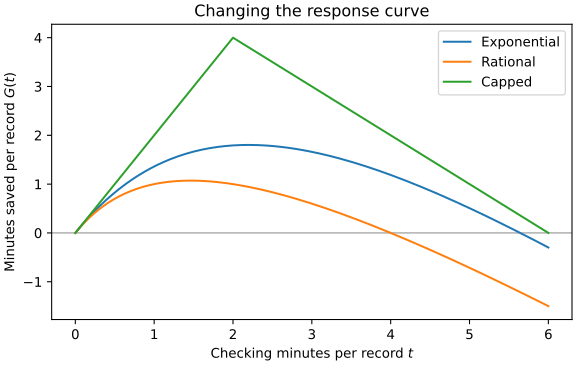
Cheaper repairs make less checking worthwhile. The same method establishes its preconditions for the revised inputs.
Try a different response without changing the argument
Return to measured, with six avoidable repair minutes per record. The
exponential curve was a modelling choice. Suppose we instead propose
This response has the same initial slope \(k\), but saturates more slowly.
RationalReview inherits the same property declarations. Replacing the
component rechecks them against the new formula and preserves the observed
detection rate. This is the replacement declaration:
class RationalReview(ExponentialReview):
    """An alternative with the same initial slope and slower saturation."""

    caught_share = (
        ExponentialReview.detection_rate
        * ExponentialReview.minutes_per_record
        / (1 + ExponentialReview.detection_rate * ExponentialReview.minutes_per_record)
    )
With the same inputs, the new marginal saving is
\(G'(t)=3/(1+t/2)^2-1\). Solving \(G'(t)=0\) on \(t\geq0\)
gives \(t_*=2(\sqrt{3}-1)\). Start from measured so the checking minutes
have not yet been fixed:
>>> from sympy import sqrt
>>> from examples.record_review import RationalReview
>>> changed = measured.replace(measured.symbols.candidate.review.response, RationalReview)
>>> changed = changed.observe({changed.symbols.candidate.review.response.minutes_per_record: 2*(sqrt(3)-1)})
>>> alternative = changed.run(review_plan)
>>> alternative.report.explain(changed.specification.stationary_maximum).verdict
'strictly true'
>>> alternative.data.minutes_per_record
2 + 4*sqrt(3)
>>> round(float(alternative.data.checking_minutes_per_record), 2)
1.46
>>> result.data.minutes_per_record == 6 + 2*log(3)
True
The candidate’s saving, workload, and derivatives now use the replaced response automatically. The same concavity argument establishes its optimum. Keeping the exponential candidate instead would fail the stationarity premise; replacing a component does not preserve conclusions about the old formula. Our earlier result remains available for comparison.
Learn from a failed replacement
A capped linear response, \(u(t)=\min(kt,1)\), looks convenient: a constant benefit per minute until all errors have been caught. At \(k=1/2\), the join is at two minutes. The left derivative is \(1/2\), while the right derivative is zero. The curve is not differentiable there, hence cannot be C².
CappedReview expresses the two parts with SymPy’s Piecewise. The first
branch applies while \(kt<1\); the final True branch covers the rest.
It inherits the original claims too:
class CappedReview(ExponentialReview):
    """A linear response with a plateau whose join violates the inherited C2 claim."""

    caught_share = Piecewise(
        (
            ExponentialReview.detection_rate * ExponentialReview.minutes_per_record,
            ExponentialReview.detection_rate * ExponentialReview.minutes_per_record < 1,
        ),
        (1, True),
    )
A failed claim is retained for inspection, so we can define this model and find out why our method cannot use it:
>>> from examples.record_review import CappedReview
>>> from modello.contrib.verification import VerificationError
>>> capped = measured.replace(measured.symbols.candidate.review.response, CappedReview)
>>> capped = capped.observe({capped.symbols.candidate.review.response.minutes_per_record: 2})
>>> capped.explain("candidate.review.response.caught_share/continuously_differentiable").verdict
'strictly false'
>>> try:
...     capped.run(review_plan)
... except VerificationError as error:
...     print(error.report.explain(capped.specification.stationary_maximum).verdict)
unresolved
Two minutes actually maximises this piecewise model: minutes saved rises before the join and falls after it. Our smooth stationary-point method cannot establish that result. A method for corners would need a different argument, such as the one-sided slopes. The capped response also has a plateau, so the original strict increase claim no longer describes it. Adopting it would require a response specification that permits this shape, as well as an appropriate method.
Evaluate a few points to explore the proposed response shape, selecting its checking-minutes input:
>>> sampled = capped.sample(
...     capped.symbols.candidate.review.response.caught_share,
...     wrt=capped.symbols.candidate.review.response.minutes_per_record, points=(1, 2, 3))
>>> tuple(float(value) for value in sampled.values)
(0.5, 1.0, 1.0)
>>> sampled.kind
'numerical observation'
A Sample records numerical evaluations. A few points cannot establish a
global property or regularity at a join, so they cannot satisfy the method’s
failed premises.
Separate a policy target from a mathematical premise
Return to the exponential plan in proposed. Suppose the team hopes to save
at least two minutes per record. That target is a goal to check, rather than
an assumption we can use to justify the plan. predicate turns the
inequality into an obligation, and consumer="review_plan" makes the method
respect it:
>>> from modello.contrib.verification import predicate
>>> ambitious = proposed.with_obligations(predicate(
...     proposed.symbols.candidate.minutes_saved_per_record >= 2,
...     name="saving_target", consumer="review_plan",
...     reason="The proposed process should save two minutes per record."))
>>> ambitious.explain("saving_target").verdict
'strictly false'
The best exponential plan saves less than the target. run(review_plan) is
blocked on this branch. To retain the measured baseline for comparison while
investigating another process, retire the experimental target explicitly:
>>> baseline = ambitious.without_obligations(
...     "saving_target", reason="Keep the measured baseline for comparison.")
>>> baseline.run(review_plan).report.explain("global_maximum").verdict
'strictly true'
>>> ambitious.explain("saving_target").verdict
'strictly false'
This removes a context-added goal. It does not remove the response’s declarations or the method’s preconditions. A real two-minute target would call for changing the process, its inputs, or the target itself.
Keep evidence with the decision
The successful result retains the report that permitted its computation.
report.explain(id) exposes conditions, domains, derivation steps, witnesses,
and checked rule premises. VerificationError similarly retains its
originating context and report when a method is blocked.
>>> import json
>>> audit_json = result.report.to_json()
>>> json.loads(audit_json)["assumptions_consistent"]
True
>>> html_page = result.report.to_html(title="Record-checking decision")
These are descriptive exports, not executable saved contexts. To export the comparisons of the three responses with the original inputs, including the blocked capped response, run the module:
$ python -m examples.record_review --output artefacts/record-review
The output contains results.json with inputs, package versions, and exact
and decimal results, plus a JSON audit and an offline HTML report for each
response. To draw both figures as well, install the optional
modello[numerics] extra and add --plot. The documentation build publishes
the results, baseline evidence,
alternative evidence, and
blocked replacement.
For a further experiment, supply a response with detection rate
Rational(1, 3) and zero error-creation rate. For
positive \(a,k\) with \(ak>1\), solving \(G'(t)=0\) gives the
positive candidate \(t_*=\log(ak)/k\). Check its premises before trusting
the new capacity.
If \(ak\leq1\), the best choice is zero checking minutes. This method checks ordinary two-sided derivatives. The nonnegative checking minutes domain supplies only one side at zero, so the endpoint check stays unresolved even when \(ak=1\) gives a formal derivative of zero. A boundary argument using the right-hand behavior is needed for this case.
Continue with writing the proof contract when you want to adapt the method, or checked bounds when a proof needs an extra argument. The verification reference covers the detailed binding, replacement, domain, and execution rules.
Change an observation: checking can introduce errors
The same response model can introduce errors as well as correct them. Its
error_creation_rate determines the share of initially correct records made
incorrect by a check: \(1-e^{-rt}\). The baseline used a zero rate.
Supply a response with an error-creation rate of one hundredth per minute. Start a fresh context with the same record estimates and detection rate, then observe the same two checking minutes as before. Each pass’s outcomes depend on the record’s state at its start:
>>> response = ExponentialReview("response", detection_rate=short.detection_rate,
...                              error_creation_rate=Rational(1, 100))
>>> extended = review_context(record, response=response)
>>> fallible = extended.observe({extended.symbols.candidate.review.response.minutes_per_record: 2})
>>> tuple(round(float(value), 4) for value in outcome_fractions(fallible.model.candidate.review))
(0.8822, 0.0632, 0.0546)
>>> round(float(fallible.model.candidate.review.introduced_error_fraction), 4)
0.0178
The corrected fraction is still 6.32% of all records. Checking also introduces errors into 1.78%, leaving 5.46% incorrect instead of the earlier 3.68%. Introduced errors are part of the remaining-error group, so the same three outcome groups still account for every record:
>>> simplify(sum(outcome_fractions(fallible.model.candidate.review)))
1
Assume an introduced error takes the same repair minutes as an original error. The existing workload now counts those repairs too. No staffing or derivative formulas need replacing:
>>> tuple(round(float(current.model.candidate.minutes_per_record), 4)
...       for current in (two_minutes, fallible))
(8.2073, 9.2765)
The old optimal checking time needs reconsidering. At \(2\log3\), the updated minutes-saved derivative is negative:
>>> old_choice = extended.observe({extended.symbols.candidate.review.response.minutes_per_record: 2 * log(3)})
>>> old_choice.model.candidate.minutes_saved_derivative.doit().is_negative
True
That point no longer satisfies the stationarity premise of review_plan.
The changed response inputs update the model’s derivatives; the verification
workflow checks the premises needed to justify a new decision.
View the same outcomes as transitions
For repeated checking, collect the review component’s two responses in a
transition matrix. Write \(a\) for introduced_error_share and
\(c\) for caught_share. They are conditional on starting correct and
incorrect respectively. corrected_fraction is \(pc\), a share of
all records.
Every ordered pair of the two states is possible, including staying in the same state. This is a complete directed graph with self-loops:
        flowchart LR
    accTitle: All correctness transitions during a check
    accDescr: Correct becomes incorrect with probability a and stays correct with probability 1 minus a. Incorrect becomes correct with probability c and stays incorrect with probability 1 minus c.
    correct(("Correct")) -->|"Error introduced: a"| incorrect(("Incorrect"))
    incorrect -->|"Error corrected: c"| correct
    correct -->|"Stays correct: 1 - a"| correct
    incorrect -->|"Stays incorrect: 1 - c"| incorrect
All four transitions for one check; outgoing probabilities from each state sum to one.
Each arrow carries a probability for one pass, here lasting two minutes. Order the states as (correct, incorrect), with rows for the current state and columns for the next:
Keep \(P\) independent of a particular response formula. A row vector \((1-p_0,p_0)\) describes the initial composition of the records: the fractions correct and incorrect. Mathematically this is a probability distribution over the two states. Multiplication by \(P\) gives the composition after one pass.
Because the shares add to one, only the incorrect share needs its own sequence. The following helper builds that sequence from the matrix product, rather than copying the review model’s formula:
from sympy import Eq, ImmutableMatrix, Lambda
from sympy.matrices import MatrixBase
from modello import Index, Recurrence, Series
def transition_recurrence(P: MatrixBase, initial_error_fraction: Expr) -> Recurrence:
    """Evolve a two-state composition using a row-stochastic transition matrix.

    Rows and columns are ordered (correct, incorrect). Conservation of records
    leaves one independent share, so a scalar recurrence represents both states.
    Probability bounds and row sums are premises to check separately.
    """
    if P.shape != (2, 2):
        raise ValueError("The record-review transition matrix must have two rows and two columns")
    n = Index("n", nonnegative=True)
    errors = Series("p", n, real=True)
    previous = ImmutableMatrix([[1 - errors[n - 1], errors[n - 1]]])
    return Recurrence(errors[n], (previous * P)[0, 1], initial={0: initial_error_fraction})
Here previous is the composition before the next pass. Its product with
P supplies the recurrence’s next incorrect share. The same law works for
any row-stochastic two-state matrix, with states ordered (correct, incorrect).
>>> from sympy import Lambda, Matrix
>>> from examples.record_review import transition_recurrence
>>> a, c = Symbol("a", nonnegative=True), Symbol("c", nonnegative=True)
>>> p0 = Symbol("p0", nonnegative=True)
>>> N = Symbol("N", integer=True, positive=True)
>>> P = Matrix([[1 - a, a], [c, 1 - c]])
>>> initial = Matrix([[1 - p0, p0]])
>>> law = transition_recurrence(P, p0)
>>> law.at(0).doit()
p0
>>> simplify(law.at(1).doit() - (initial * P)[0, 1])
0
>>> response_after_N = law.at(N).doit()
Recurrence has derived the response at an arbitrary pass count. In a
more readable form, it is
The calculation used nonnegative \(a,c\). Their probability interpretation also needs \(a,c\leq1\) and \(0\leq p_0\leq1\). For \(0<a+c<2\), the power tends to zero, leaving the stationary fraction \(a/(a+c)\). A matrix that swaps the two states on every pass has \(a=c=1\) and can oscillate; a stationary fraction alone does not establish convergence. If both transition shares are zero, the matrix is the identity and every pass leaves the initial composition unchanged.
Lambda packages the derived expression as a symbolic function of the two
transition shares, initial composition, and pass count. Choosing matrix
entries is now enough to choose the response:
>>> finite_response = Lambda((a, c, p0, N), response_after_N)
>>> finite_response(0, 0, p0, 5)
p0
>>> from examples.record_review import review_transition_matrix
>>> review_P = review_transition_matrix(extended.symbols.candidate.review.response)
>>> observed_P = review_P.applyfunc(fallible.expression)
>>> after_one = finite_response(observed_P[0, 1], observed_P[1, 0],
...                             record.error_fraction, 1)
>>> simplify(after_one - fallible.model.candidate.review.remaining_error_fraction)
0
The existing response is one choice of matrix entries. Its one-pass result
agrees with ReviewModel. Keep those entries fixed to ask about repeated
two-minute passes.
RepeatedReview reuses the same recurrence helper. It contains the existing
review model, relates total checking time to pass duration, and queries the
recurrence at the inferred pass count:
class RepeatedReview(Modello):
    """Infer pass count and evolve record composition with the same matrix law."""

    review = component(ReviewModel)
    passes = InstanceDummy("N", integer=True, nonnegative=True)
    checking_minutes_per_record = passes * review.response.minutes_per_record
    progression = transition_recurrence(
        review_transition_matrix(review.response),
        review.record.error_fraction,
    )
    final_error_fraction = progression.at(passes)
>>> from examples.record_review import RepeatedReview
>>> repeated = VerificationContext.for_model(RepeatedReview, "four checking minutes")
>>> repeated = repeated.observe({
...     repeated.symbols.review.record: record,
...     repeated.symbols.review.response: response,
...     repeated.symbols.review.response.minutes_per_record: 2,
...     repeated.symbols.checking_minutes_per_record: 4,
... })
>>> repeated.model.passes
2
>>> round(float(repeated.model.final_error_fraction.doit()), 4)
0.0388
>>> simplify(repeated.model.final_error_fraction.doit()
...          - finite_response(observed_P[0, 1], observed_P[1, 0],
...                            record.error_fraction, repeated.model.passes))
0
For zero passes the recurrence returns the initial composition. This avoids building a finite history merely to query its last value. Total staff time still includes entry and repair work as well as checking.
The same matrix recurrence also has a long-run limit for these observed probabilities:
>>> long_run_errors = limit(
...     finite_response(observed_P[0, 1], observed_P[1, 0], record.error_fraction, N),
...     N, S.Infinity)
>>> round(float(long_run_errors), 4)
0.0304
We can ask the original outcome model for its equilibrium too. Reuse its components and join the error fractions before and after a pass:
class ReviewEquilibrium(Modello):
    """Infer an error fraction unchanged by one pass of fallible review."""

    review = component(ReviewModel)
    error_fraction = review.record.error_fraction
    error_fraction = review.remaining_error_fraction
>>> from examples.record_review import ReviewEquilibrium
>>> equilibrium = ReviewEquilibrium("unchanged quality", **{
...     "review.response": response,
...     "review.response.minutes_per_record": 2,
... })
>>> simplify(equilibrium.error_fraction - long_run_errors)
0
The equilibrium equality identifies a fixed point. The recurrence explains when repeated passes approach it.
Check the transition properties in the same context
The probability premises belong to the chosen matrix. Give them a Python schema so an editor can complete their names and a type checker can reject a missing attribute. The example uses an ordinary frozen dataclass:
@dataclass(frozen=True)
class ReviewSpecification:
    """Named declarations for the selected stage of the investigation."""

    stationary_maximum: InferenceRule
    nonnegative_entries: tuple[tuple[Obligation, ...], ...] = ()
    normalized_rows: tuple[Obligation, ...] = ()
    positive_entries: tuple[tuple[Obligation, ...], ...] = ()
The same catalog already names the stationary-point inference rule. Its tuple fields can hold obligations for a matrix of any finite shape. A factory fills those fields from the current model symbols:
def transition_specification(symbols: ReviewPlanning, *, mixing: bool = False) -> ReviewSpecification:
    """Name the matrix's probability premises, with optional convergence goals."""
    P = review_transition_matrix(symbols.candidate.review.response)
    return ReviewSpecification(
        stationary_maximum=STATIONARY_MAXIMUM,
        nonnegative_entries=tuple(tuple(nonnegative(entry) for entry in P.row(i)) for i in range(P.rows)),
        normalized_rows=tuple(equal_to(sum(P.row(i)), 1) for i in range(P.rows)),
        positive_entries=tuple(
            tuple(positive(entry, consumer="convergence") for entry in P.row(i)) for i in range(P.rows)
        )
        if mixing
        else (),
    )
with_specification binds the factory to the context. specification
returns its typed catalog; obligations and rules expose the active
context-level goals and inference rules as read-only tuples. The catalog’s
field names and tuple positions supply report IDs automatically:
>>> from examples.record_review import transition_specification
>>> transitions = extended.with_specification(transition_specification)
>>> checked = transitions.observe({transitions.symbols.candidate.review.response.minutes_per_record: 2})
>>> checked.explain(checked.specification.nonnegative_entries[0][1]).verdict
'strictly true'
>>> len(checked.obligations), len(checked.rules)
(6, 1)
>>> review_P.applyfunc(checked.expression) == observed_P
True
These obligations describe a row-stochastic matrix: entries are nonnegative and each row sums to one. They also bound every entry above by one.
For convergence to a unique stationary distribution, a useful sufficient condition here is that all four entries are strictly positive. It gives \(0<a,c<1\) and therefore \(|1-a-c|<1\). Add those stronger obligations when using that argument:
>>> mixing = checked.with_specification(
...     lambda symbols: transition_specification(symbols, mixing=True))
>>> mixing.explain(mixing.specification.positive_entries[0][1]).verdict
'strictly true'
These are proof goals; they do not automatically guard native SymPy
calculations. A computation that relies on them can list them as a
Method’s preconditions. An initial composition also needs nonnegative
entries summing to one.
Derive a continuous response from shorter steps
The limit above spends more time checking as it adds passes. A different question keeps the total checking time \(t\) fixed and divides it into more steps. This lets a record change state more than once during one check: an error can be corrected and another introduced afterwards.
For a short step lasting \(h\) minutes, take the correction share to be \(kh\) and the error-introduction share to be \(rh\):
For nonnegative rates, this is a probability matrix once the steps are short enough that \(rh\leq1\) and \(kh\leq1\). The recurrence stays the same: choose these entries, evaluate at \(N\) steps, and let \(N\to\infty\) at fixed \(t\).
derive_continuous_transitions performs those operations. It first derives
the response for independent nonnegative \(a,c\), then uses Lambda to
supply the short-step entries and SymPy to take the limit. Starting wholly
correct or wholly incorrect gives the two rows of the continuous matrix.
The explicit zero-total-rate branch retains the degenerate limit; when both
physical rates are zero, the result is the identity matrix.
def derive_continuous_transitions(
    minutes_per_record: Expr, detection_rate: Expr, error_creation_rate: Expr
) -> ImmutableMatrix:
    """Derive a continuous two-state response from increasingly short checks.

    First solve the recurrence for independent, nonnegative transition shares.
    Then parameterize those shares by short-step rates and take the limit at
    fixed total checking time. The zero-total-rate branch retains the affine
    limit too; with physical nonnegative rates this is the identity matrix.
    """
    a, c = (Dummy(name, nonnegative=True) for name in ("a", "c"))
    initial = Dummy("p", real=True)
    steps = Dummy("N", integer=True, positive=True)
    P = ImmutableMatrix([[1 - a, a], [c, 1 - c]])
    discrete = Lambda((a, c, initial), transition_recurrence(P, initial).at(steps).doit())

    minutes, correction, creation = (Dummy(name, positive=True) for name in ("t", "k", "r"))
    step = ImmutableMatrix(
        [
            [1 - creation * minutes / steps, creation * minutes / steps],
            [correction * minutes / steps, 1 - correction * minutes / steps],
        ]
    )
    after_steps = discrete(step[0, 1], step[1, 0], initial)
    continuous = Lambda((minutes, correction, creation, initial), simplify(limit(after_steps, steps, S.Infinity)))
    rows = []
    for starting_errors in (S.Zero, S.One):
        errors = Piecewise(
            (starting_errors + error_creation_rate * minutes_per_record, Eq(detection_rate + error_creation_rate, 0)),
            (continuous(minutes_per_record, detection_rate, error_creation_rate, starting_errors), True),
        )
        rows.append([1 - errors, errors])
    return ImmutableMatrix(rows).applyfunc(simplify)
For \(k>0,r\geq0\), the derived composition after \(t\) minutes is
The two matrix entries needed by the review model are
These account for both directions throughout the check. They replace the
earlier assumption of separate responses 1-exp(-r*t) and 1-exp(-k*t)
for one pass. With \(r=0\), the introduced share is zero and the caught
share is exactly the original 1-exp(-k*t).
The entries describe the state at the end of checking. The share \(a(t)\) starts correct and ends incorrect; \(c(t)\) starts incorrect and ends correct. Any intervening changes of state are already included.
The extension uses those cells directly. The matrix below is expressed in
the parent model’s inputs, so inheritance rebinds its entries along with the
existing property claims. Only detection_rate is redeclared, to strengthen
its domain to positive rates; checking minutes and the error-creation rate
are inherited:
# The parent inputs keep their identities when its response equations change.
P = derive_continuous_transitions(
    ExponentialReview.minutes_per_record, ExponentialReview.detection_rate, ExponentialReview.error_creation_rate
)


class ContinuousReview(ExponentialReview):
    """Allow correction and error creation throughout a single check, with k > 0."""

    # Refine this input's domain; the other inputs and claims are inherited.
    detection_rate = InstanceDummy("k", positive=True)
    introduced_error_share = P[0, 1]
    caught_share = P[1, 0]
Replace the response in the context that already carries our record estimates, rates, and probability obligations. Its specification factory runs with the replacement’s symbols, so the typed catalog follows the new response. The outcome and workload equations stay the same:
>>> from examples.record_review import ContinuousReview
>>> continuous = transitions.replace(transitions.symbols.candidate.review.response, ContinuousReview)
>>> continuous = continuous.observe({continuous.symbols.candidate.review.response.minutes_per_record: 2})
>>> round(float(continuous.model.candidate.review.remaining_error_fraction), 4)
0.0486
>>> continuous.explain(continuous.specification.nonnegative_entries[0][1]).verdict
'strictly true'
>>> continuous.explain("candidate.review.response.caught_share/continuously_differentiable").verdict
'strictly true'
>>> recovered = two_minutes.replace(two_minutes.symbols.candidate.review.response, ContinuousReview)
>>> simplify(recovered.model.candidate.minutes_per_record
...          - two_minutes.model.candidate.minutes_per_record)
0
The coupled response leaves about 4.86% incorrect after two minutes, compared with 5.46% for the earlier one-pass assumption. Its long-time error fraction is \(r/(k+r)\), here \(1/51\) or about 1.96%. The zero-error-creation baseline is recovered without changes to the workload model.
The matrix now drives finite-pass inference, the continuous limit, and the replacement response. The same context can then check the premises needed for a workload or optimality calculation with that response.